Introduction to Numerical Python
What is “Numerical Python”?
-
A collection of many libraries to make numerical computation easier.
-
NumPy: $N$-dimensional arrays, fast linear algebra
-
SciPy: Optimization, interpolation, statistics, special functions, …
-
SymPy: Symbolic computation
-
MatPlotLib: Data visualization, plotting
-
Pandas: Data analysis
-
-
Various others: TensorFlow, PyTorch for Machine Learning, …
Why NumPy?
-
Python Sucks
-
Python is slow (interpreted, dynamically typed).
-
Parallelization limited by the Global Interpreter Lock
-
-
Long live Python
-
Use multiprocessing / memhive to sidestep the Global Interpreter Lock
-
Use fast optimized libraries to do the bulk of the work. (
NumPy, etc) -
Python provides an easy to learn/use interface.
-
Numpy Fundamentals
-
Python
list: One dimensional, can expand / grow. -
NumPy
array(akandarray): Fixed size; multiple dimensions.>>> a = np.array( [ [1,2,3], [4,5,6] ] ) >>> a array([[1, 2, 3], [4, 5, 6]]) >>> a.shape (2, 3) >>> a[1,2] np.int64(6) -
Array operations: Operators act on arrays element-wise:
>>> a ** 2
array([[ 1,  4,  9],
       [16, 25, 36]])
>>> a + 1
array([[2, 3, 4],
       [5, 6, 7]])
Slicing / iterating
-
Slicing works as expected
a[1, :] # [4, 5, 6] (second row) a[:, 0] # [1, 4] (first column) a[1] # Equivalent to a[1, :] -
Use
a[..., m:n:s, ...]in any position- Extracts every $s^\text{th}$ element from
m(inclusive) ton(exclusive).
- Extracts every $s^\text{th}$ element from
-
Iterating is done over the first axis:
for r in a: # iterates over rows a[0], a[1], ...
for x in a[1]: # interates over column a[1, 0], a[1, 1], ...
Universal functions
-
mathfunctions don’t act on arrays:math.sin(a) # Error -
NumPyfunctions act on arrays element wise:np.sin(a) # gives [ sin(a[0]), sin(a[1]), ... ] -
NumPyfunctions also act on scalarsnp.sin(0) # works math.sin(0) # works -
See
NumPydocumentation on universal functions
Extremely convenient for numerical work
-
Regular python
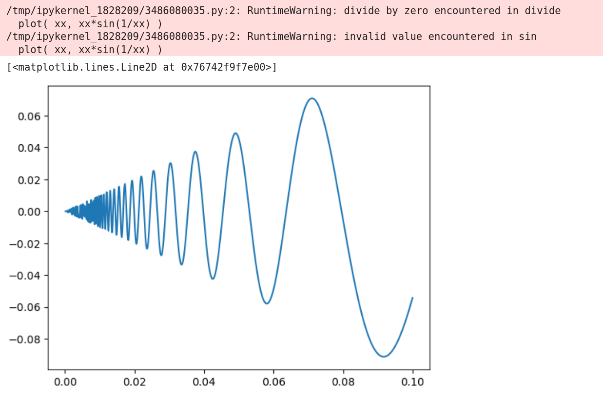
for i in range( N ): x = 0.1*i/N plot( x, x*math.sin(1/x) ) # Division by 0 exception -
NumPy:xx = np.linspace( 0, 2*pi, N ) plot( xx, xx*np.sin(1/xx) ) # Runtime warning, but works
Using NumPy
-
Option 1:
%pylab inline(Quick and dirtyMatLabtype environment)- Imports all functions from
matplotlib.pylabandnumpy - Replaces Python
sumwithnumpy.sum - Depreciated; but very useful if you just want a quick plot / scratch.
- Imports all functions from
-
Option 2: Import the functions you want.
%matplotlib inline
# Another option is `%matplotlib widget`
import numpy as np, matplotlib as mpl, scipy as sp
from matplotlib import pylab, mlab, pyplot as plt
from matplotlib.pylab import plot, scatter, contour
from tqdm.notebook import tqdm, trange

from numpy import sqrt, pi, exp, log, floor, ceil, sin, cos
from numpy.linalg import norm

rng = np.random.default_rng()
Monte Carlo compute $\pi$
-
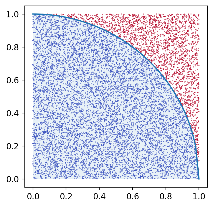
$U \sim \Unif([0,1]^2)$
-
$\P( \abs{U} < 1 ) = \frac{\pi}{4}$
-
Compute $\displaystyle \frac{1}{N} \sum_1^N \one_{\set{\abs{U_i} < 1}}$.
- Approximates $\pi$ with an $O(1/\sqrt{N})$ error
Checking performance
-
Set
N = 10**7 -
“First” implementation: (took 33.31s)
n_inside = 0 for i in trange(N): (U1, U2) = (rng.uniform(), rng.uniform()) if sqrt(U1**2 + U2**2) < 1: n_inside += 1 -
Implementation with
NumPyfunctions: (took 0.195s)U = rng.uniform( size=(2, N) ) n_inside = np.sum( norm( U, axis=0 ) < 1 ) -
Use library functions as much as you can.
-
Avoid Python loops as much as possible.
Don’t run out of memory
-
Easy to set $N = 10^9$, and run
U = rng.uniform( size=(2, N) ) -
Takes
15Gbmemory to store. May crash your computer -
Run code in chunks:
N = 10**9 M = 1000 n_inside = 0 for i in trange(M): U = rng.uniform( size=(2, N//M) ) n_inside += np.sum( norm( U, axis=0 ) < 1 ) -
Can trivially parallelize chunks.
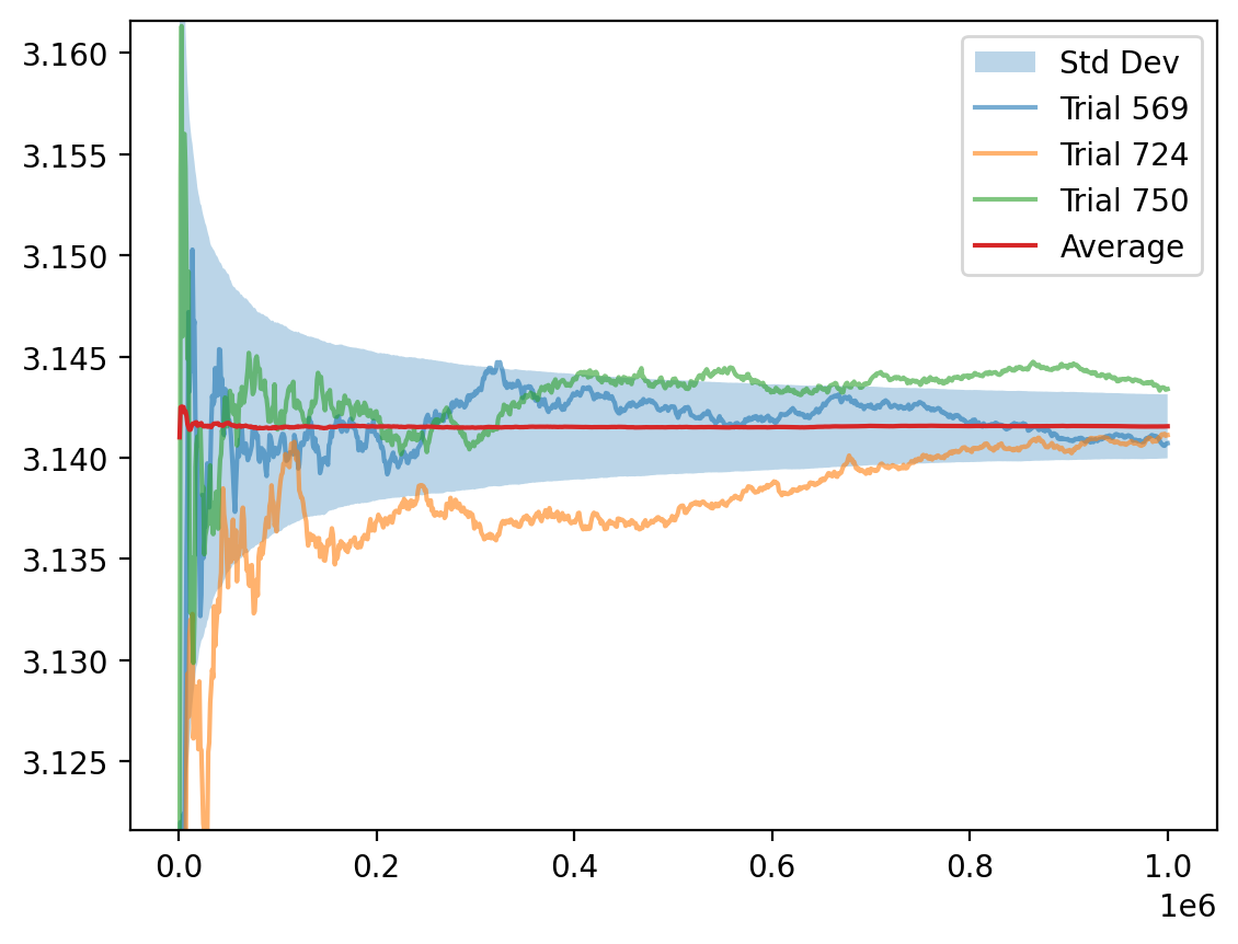
Estimate of $\pi$ as $N \to \infty$.
for n in trange( n_iters ):
    U = rng.uniform( size=(2, M, n_trials) )
    n_inside = np.sum( norm( U, axis=0 ) < 1, axis=0 )
    hat_π[n] = 4*n_inside
hat_π = (np.cumsum( hat_π, axis=0 ).T / NN).T
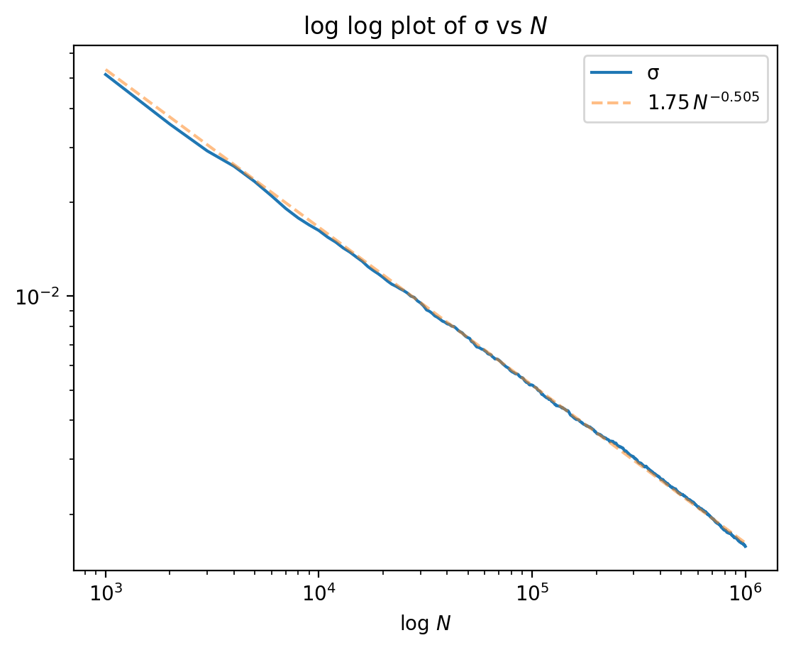
Checking error scales like $O(1/\sqrt{N})$
# Use `polyfit` to fit $\log(σ)$ to $a + b N$.
plt.loglog( NN, σ, label='σ' )

a = np.polyfit( log(NN), log(σ), 1 )
plt.loglog( NN, exp( a[0]*log(NN) + a[1] ), '--',
    alpha=.5, label=f'${exp(a[1]):.2f}\\, N^{{{a[0]:.3f}}}$' )
Volume of a $d$-dimensional ball
-
Suppose $U \sim \Unif( [0, 1]^d )$. Then $\displaystyle \P( \abs{U} < 1 ) = \frac{\vol( B(0, 1) )}{2^d}$
-
Exact formula: $\displaystyle \vol(B(0, 1)) = \frac{\pi^{d/2}}{\Gamma(\frac{d}{2}+1)}$
-
Easy to implement:
for d in trange( 1, D ):
    vol[d] = pi**(d/2) / sp.special.gamma( d/2 + 1 )

    U = rng.uniform( size=(d, N) )
    n_inside = np.sum( norm(U, axis=0) < 1 )
    hat_vol[d] = 2**d * n_inside/N
Curse of dimensionality
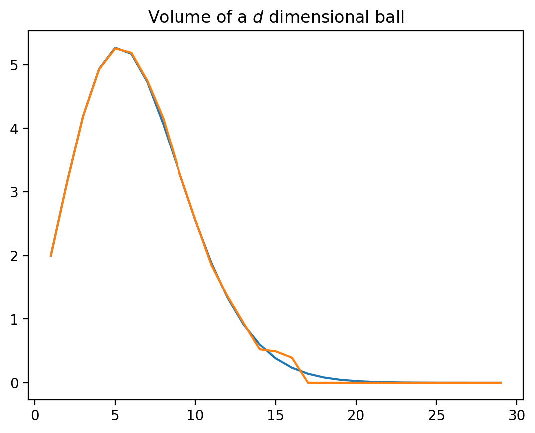
Simulations don’t find even one point inside $B(0,1)$ in high dimensions.
Problem: Generate a Rejection Sample plot
-
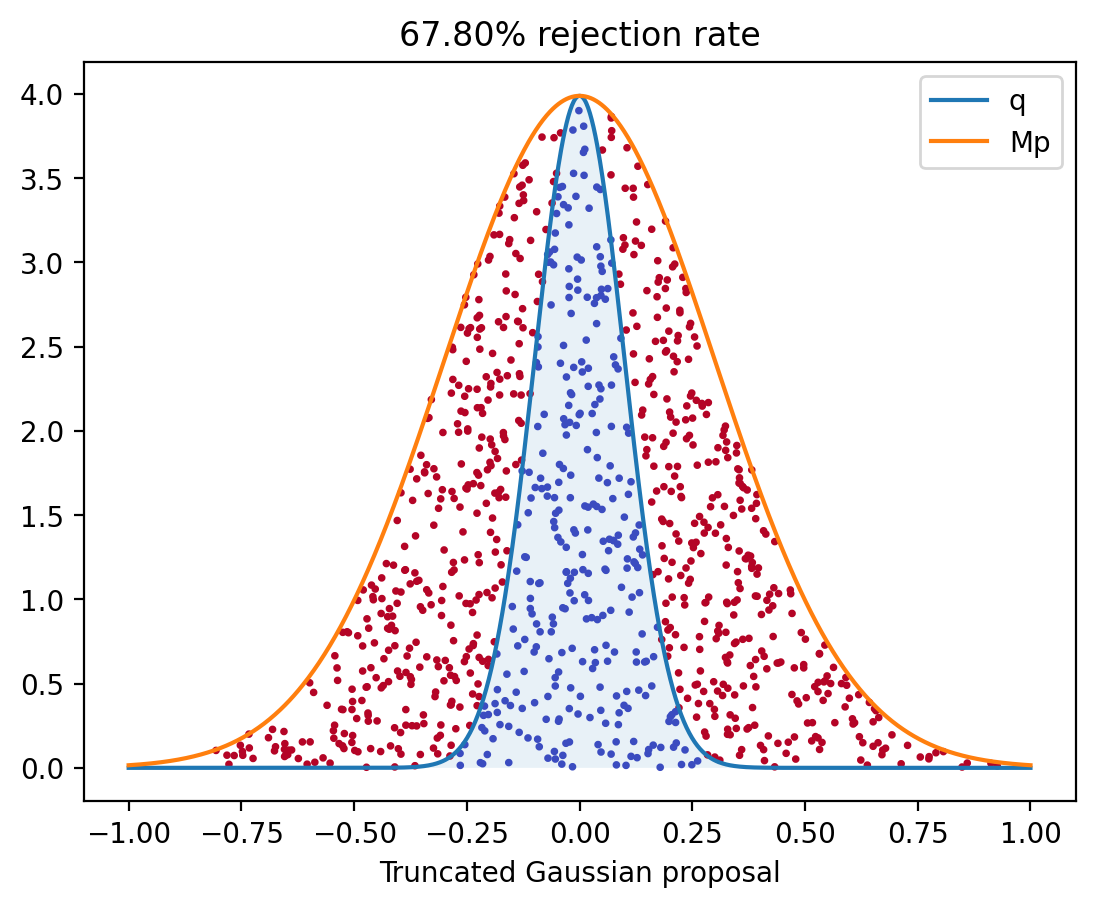
Points above the graph of $q$ (in red) are rejected -
Sample one $X \sim p$, one $U \sim \Unif([0, 1])$.
-
Set
color=redif $Mp(X) > q(X)$. -
Set
color=blueotherwise. -
plot( X, M p(X), color ) -
Repeat 1,000 times.
-
-
Try to vectorize this and plot without looping.
Problem: Numerically finding the PDF/CDF
-
Say
XhasNsamples from some distribution. -
Problem: Numerically approximate the CDF and PDF.
-
Algorithm for computing the CDF:
-
Say the points are $x_1, \dots, x_N$ with $x_1 < x_2 \cdots < x_N$.
-
Know $F(x_k) = k/N$. Find $F$ at other points by interpolating.
-
-
Implement this so you get acquainted with NumPy/SciPy:
- Use UnivariateSpline for interpolation
(see also LSQUnivariateSpline.)
- Tune the smoothing factor
sto get good results.
- Tune the smoothing factor
- Use pad to pad the data
- Use scipy.stats for the exact PDF/CDF of various distributions.
- Use UnivariateSpline for interpolation
(see also LSQUnivariateSpline.)
Numerical approximation of the CDF
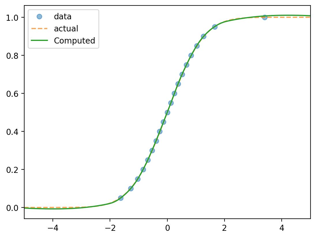
Data: 10,000 samples from $N(0, 1)$
Numerically finding the PDF
-
Option 1: Differentiate the CDF (use UnivariateSpline.derivate)
-
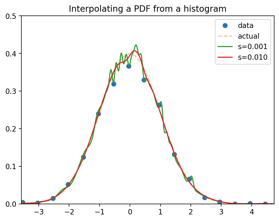
Option 2: Create a histogram.
-
numpy.histogram divides the data into bins
-
Assume the PDF at bin midpoints is proportional to the counts
-
Interpolate and smooth.
-
Numerical approximation of the PDF
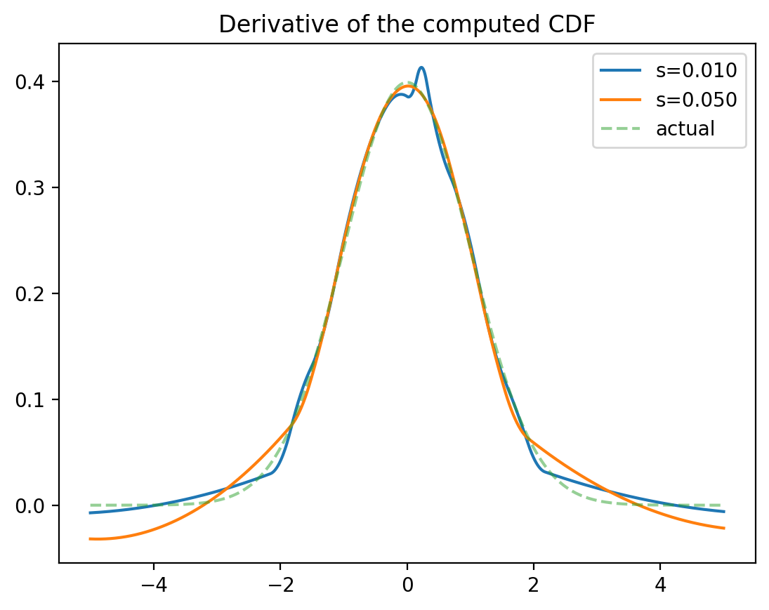
Few concluding tips
-
Jupyter Notebooks make it easy to run simulations interactively.
-
Online documentation is excellent.
-
Shift+Tab/Ctrl+I/ right click for contextual help -
Use library functions. Don’t reinvent the wheel.
scipy.randomsamples from most common distributionsscipy.interpolatehas curve fitting / interpolation functionsscipy.linalg,numpy.linalgvarious linear algebra functions
-
Use vectorized functions; avoid loops as much as possible.
-
Notebook with code from these slides is here.