Basic Sampling Algorithms.
Uniform sampling
Our goal is now to build a collection of distributions we can effectively sample from.
Question 1. Suppose you have a random bit generator that returns either $0$ or $1$ with probability $1/2$, and is independent of all previous results.
-
How do you generate a uniformly random number $N \in \set{0, \dots, 2^N -1 }$ (i.e. how do you sample from the uniform distribution on $\set{0, \dots, 2^N - 1}$
-
How do you sample from the uniform distribution on $\set{0, \dots, M}$, where $M$ is not necessarily a power of $2$?
-
How do you sample from the uniform distribution on $[0, 1]$?
Transformation Methods
The idea behind transformation methods is to start with a random variable $X$ you can effectively simulate, and find a transformation $T$ so that $T(X)$ follows your desired distribution.
Lemma 2. Suppose $\Omega \subseteq \R^d$, and $T \colon \Omega \to \R^d$ is some $C^1$, injective transformation for which with $\det{DT}$ never vanishes. If $X$ is a $\Omega$-valued random variable with probability density function $p$, then $T(X)$ is an $\R^d$ valued random variable with probability density function $q$, where \begin{equation} q = p \circ T^{-1} \abs{\det DT^{-1}} \,. \end{equation}
Remark 3. Here $T^{-1}$ is the inverse of the function $T$, and $DT^{-1}$ is the Jacobian matrix of $T^{-1}$.
Remark 4. Recall, we say $p$ is the probability density function of a $\R^d$ valued random variable $X$ if for every (nice) set $A \subseteq \R^d$, we have \begin{equation} \P(X \in A) = \int_A p(x) \, dx\,. \end{equation} When $d = 1$ the above is a $1$-dimensional Riemann integral, when $d = 2$, the above is a area integral, and when $d = 3$ the above is a volume integral. In dimensions higher than $3$ this is a Lebesgue integral, and can be thought of as $d$ iterated integrals. No matter what the dimension is, we will always only use one integral sign, and never write $\iint$ or $\iiint$.
Proof. Done in class.
Proposition 5 (Box Mueller). Suppose $U = (U_1, U_2)$ is uniformly distributed on $(0, 1)^2$. Set \begin{gather} Z_1 = \sqrt{-2 \ln U_1} \cos( 2 \pi U_2 )\,, \\ Z_2 = \sqrt{-2 \ln U_1} \sin( 2 \pi U_2 )\,. \end{gather} Then $Z = (Z_1, Z_2)$ is a standard two dimensional normal.
Let $F$ be the CDF of a target PDF $q$. If $U \sim \Unif([0, 1])$, then $F^{-1}(U)$ is a random variable with PDF $q$.
Proof. Follows from Lemma 2.
Remark 7. If $q$ is a PDF for which $F^{-1}$ can be computed easily, then the inversion method is a very efficient method of sampling from $q$.
Example 8. Consider the exponential distribution with parameter $\lambda$. The CDF and inverse CDF can be computed to be \begin{equation} F(x) = \P(X \leq x) = 1 - e^{-\lambda x} \,, \qquad F^{-1}(x) = \frac{-\ln(1-x)}{\lambda} \,. \end{equation} Thus if $U \sim \Unif([0, 1])$ then $-\ln( 1 - U ) / \lambda \sim \Exp(\lambda)$.
Let $q = q(x_1, x_2)$ be a two dimensional target PDF. Let $q_1, F_1$ be the PDF and CDF of the first marginal: Explicitly, \begin{gather} q_1(x_1) = \int_\R q(x_1, x_2) \, d x_2 \qquad\text{and}\qquad F_1(x_1) %= \P( X_1 \leq x_1 ) = \int_{x \leq x_1} q_1(x) \, dx \,. \end{gather} Let $F_{2, x_1}$ be the CDF of the second marginal conditioned on $x_1$. That is, \begin{equation} F_{2, x_1}(x_2) %= \text{“}\P( X_2 \leq x_2 \given X_1 = x_1 )\text{”} = \frac{1}{q_1(x_1)} \int_{-\infty}^{x_2} q(x_1, y) \, dy \,. \end{equation} Define the transformation $T \colon (0, 1)^2 \to \R^2$ by \begin{equation} T(u_1, u_2) = ( F_1^{-1}(u_1), F_{2, x_1}^{-1}(u_2) ) \,, \end{equation} where \begin{equation} x_1 = F_1^{-1}(u_1) \,. \end{equation} If $U = (U_1, U_2)$ is uniformly distributed random variable on $(0, 1)^2$, then the PDF of $T(U)$ is $q$.
Remark 10. The notation $F_{2, x_1}^{-1}$, denotes the inverse of the function $y \mapsto F_{2, x_1}(y)$ for a fixed $x_1$. We also implicitly assume $q_1 \neq 0$, otherwise we restrict the domain accordingly.
Remark 11. The Knothe–Rosenblatt rearrangement can be used to efficiently sample from two dimensional distributions, provided the inverse CDFs $F_1^{-1}$, $F_{2, x_1}^{-1}$ can be computed.
Remark 12. This can easily be generalized to higher dimensions by setting \begin{equation} T(u_1, u_2, u_3 ) = ( F_1^{-1}(u_1), F_{2, x_1}^{-1}(u_2), F_{3, x_1, x_2}^{-1}(x_3), \dots ) \,, \end{equation} where \begin{equation} x_1 = F_1^{-1}(u_1)\,, \quad x_2 = F_{2, x_1}^{-1}(u_2) \quad \dots \,. \end{equation}
Rejection sampling
Suppose we can draw independent samples from a proposal distribution with density $p$, and the uniform distribution, then we can sample from any target distribution $q$ as long as $\max q/p < \infty$.
Require Proposal PDF $p$, target PDF $q$, with $M = \max q/p < \infty$.
-
Choose independent $X\sim p$, $U \sim \Unif( [0, 1] )$
-
If $U < q(X) / (M p(X) )$, then return $X$. Otherwise go back to the previous step.
Remark 14. This proposition shows that the output of this algorithm has distribution $q$, and this lemma shows that it returns (on average) in $M$ steps.
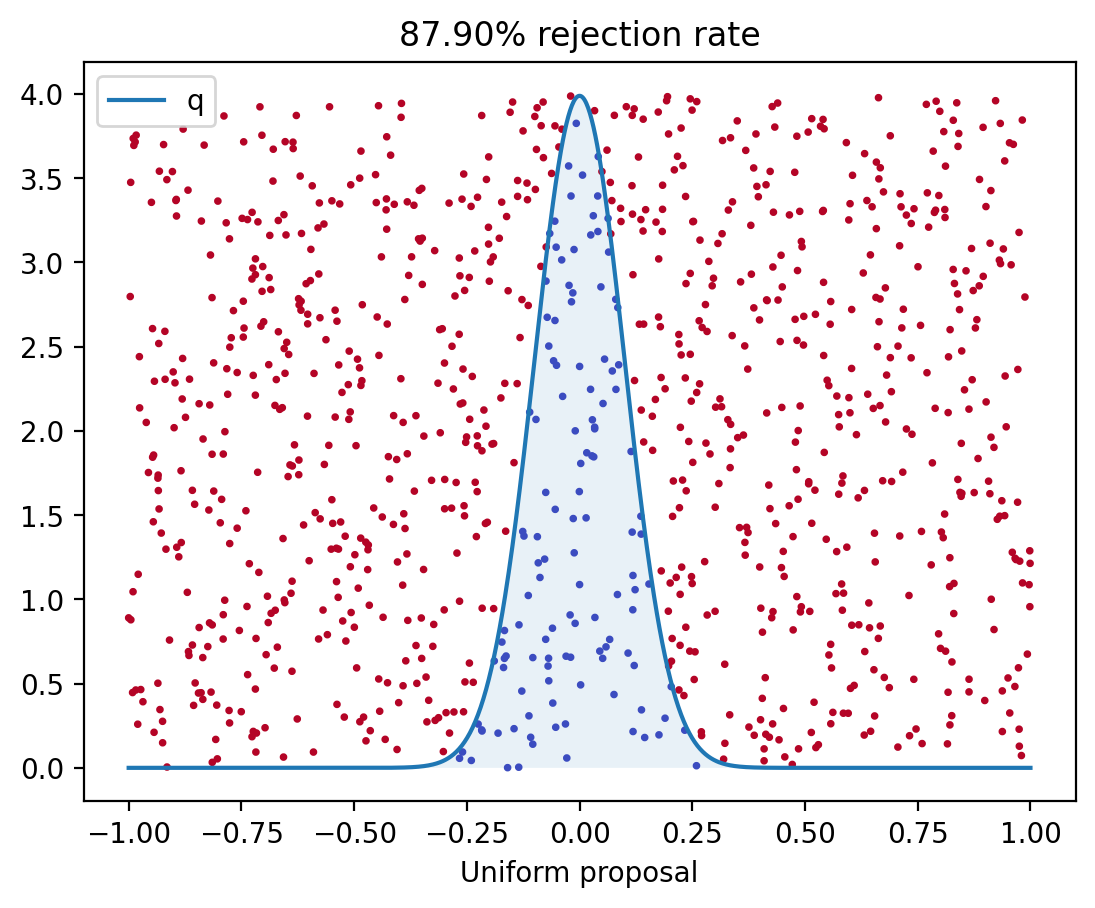
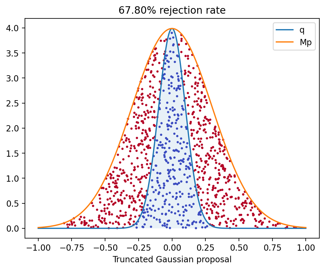
The algorithm is easy to understand with a picture: Let $M = \max q/p$. Simulate $X_1$, …, $X_N$ independently from the distribution $p$. Simulate $U_1$, …, $U_N$ independently from $\Unif([0,1])$. Plot the points $(X_i, U_i M p(X_i) )$. Throw away all the points that are above the graph of $q$. Two examples of this are shown in here.


Proposition 15. Let $X_n$ be i.i.d. random variables whose common distribution has density $p$. Let $U_n$ be independent, $\Unif([0,1])$ distributed random variables. Define \begin{equation} N = \min \set[\Big]{n \st U_n \leq \frac{q(X_n)}{M p(X_n)} } \quad\text{where}\quad M = \max_x \set[\Big]{ \frac{q(x)}{p(x)} } \,, \end{equation} and set $Y = X_N$. Then the PDF of $Y$ is $q$.
Proof. Done in class.
Lemma 16. If $N$ is as in Proposition 15, then $\P(N = 1) = 1/M$ and $\E N = M$. (In other words, to produce one sample from $q$, you have to draw on average $M$ samples from $p$.)
The computational cost of rejection sampling typically grows exponentially with the dimension. That is if $p, q$ are $d$-dimensional distributions, you can in general expect $\max q/p$ to be exponentially large in $d$. A simple illustration is if we try to rejection sample the uniform distribution on the unit ball $B(0, 1) \subseteq \R^d$, starting with the uniform distribution on a larger ball; say $B(0, 2)$. In this case \begin{equation} M = \max \frac{q}{p} = \frac{ \vol(B(0, 2)) }{ \vol(B(0, 1)) } = 2^d \,. \end{equation}
Another example is rejection sampling the uniform distribution $B(0, 1)$ starting from the uniform distribution on the unit cube $[-1, 1]^d$. In this case \begin{equation} M = \max \frac{q}{p} = \frac{2^d}{\vol(B(0, 1))} = \frac{2^d \Gamma(1 + n/2) }{\pi^{d/2}} \approx \sqrt{d \pi} \paren[\Big]{ \frac{2d}{\pi e}}^{d/2} \,, \end{equation} which grows exponentially with $d$.
Remark 18. Rejection sampling can almost always be used; but before using it try and estimate $M$. If it’s too large, rejection sampling might not work in practical amounts of time.