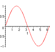
Suppose an animal population oscillates sinusoidally from a low of 700 on January 1 and a high

of 900 on July 1. Find a formula for the population at any point in time during the year. Plot the function.

We found that the function is P(t)=800+100*sin[Pi/6(t-3)]

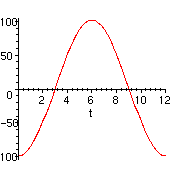
Start with the graph of sin(t):

> plot(sin(t),t=0..2*Pi);

Horizontally stretch the graph so that it's period is 12 months.

> plot(sin((Pi/6)*t),t=0..12);

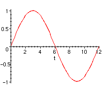
Next shift the graph 3 units to the right.

> plot(sin((Pi/6)*(t-3)),t=0..12);

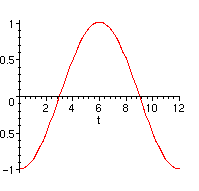
Next vertically stretch it by a factor of 100:

> plot(100*sin((Pi/6)*(t-3)),t=0..12);

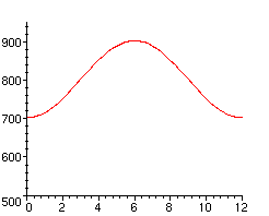
Next shift it vertically up 800 units:

> plot(800+100*sin((Pi/6)*(t-3)),t=0..12);

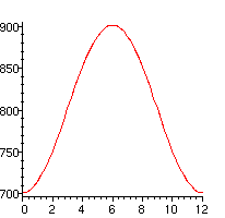
Finally let's change the range to remind ourselves that the graph doesn't start at the origin:

> plot(800+100*sin((Pi/6)*(t-3)),t=0..12,P=500..950);

>

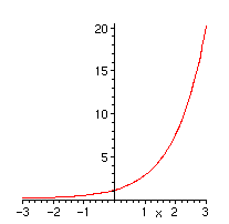
Let's plot the exponential. Note that unlike the graphing calculators, to get the number e we must type exp(1) NOT e^(1).

over the interval [-3,3]?

> plot(exp(x),x=-3..3);

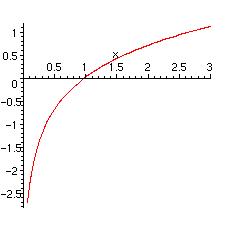
Now let's plot the graph of the natural logarithm.

> plot(ln(x),x=0..3);

Maple can solve some equations analytically:

> eq:=x^2-5*x-11;

> sol:=solve(eq=2,x);

You can access the solutions by giving them names and using the square brackets as follows:

> sol[1];

> sol[2];

> solve(exp(3*x)=2,x);

Sometimes Maple will miss a solution. For instance if you take a rational function.

> rat_eq:=x^2+1/x-1/x^2;

If you were to solve this by hand you would first get a common denominator and set the numerator equal to zero. Recall that Maple gets a common denominator using simplify:

> simplify(%);

> soln:=solve(rat_eq=0);

This means that Maple cannot do it analytically. Note however that it arrived at the same expression that we got by finding a common denominator. So try the command fsolve to get approximate roots.

> soln:=fsolve(rat_eq=0,x);

You can check graphically that it missed a positive root.

> plot(rat_eq,x=-2..2,y=-20..20);

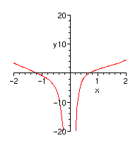
To find that root tell Maple to look in the interval (0,1):

> fsolve(rat_eq=0,x,x=0..1);

Note that Maple does not distinguish between log and ln.

> evalf(log(3));

> evalf(ln(3));

To get log base 10 of 3 you need to use the conversion formula. Basically divide by log(10):

> evalf(ln(3)/ln(10));

In class we solved the equation log(3x+2)+log(x-1)=1 analytically. Let's see if maple get the same answer:

> solve(log(3*x+2)+log(x-1)=log(10),x);

> evalf(%);

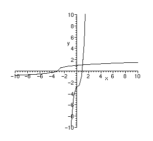
To get the inverse of a function with maple, first plot the graph of the original function and see if it passes

the horizontal line test:

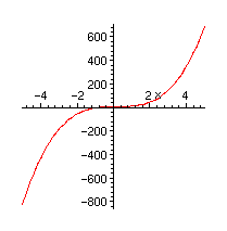
> g:=x->6*x^3-3*x^2+x-3;

> plot(g(x),x=-5..5);

Next recall the method of finding the inverse. Interchange x and y and solve for y. You will get several answers some of which involve complex numbers like I. Ignore these for now. Just take the first answer.

> g_inv:=solve(x=g(y),y);

When you run the previous command you get a huge mess. Don't worry about understanding it now.

You should see that the graph of the original function and its inverse are related by a reflection in the line y=x:

> plot({g(x),g_inv},x=-10..10,y=-10..10,color=black);