It is often useful to find a formula for a sequence of numbers. Having such a formula allows us to predict other numbers in the sequence, see how quickly the sequence grows, explore the mathematical properties of the sequence, and sometimes find relationships between one sequence and another. If the sequence is counting something (for example, the number of polyominoes of each area), having a formula helps us to catch omissions or duplicates if we are trying to make a complete list.
If we have a (partial) sequence of numbers, how can we guess a formula for it? There is no method that will always work for all sequences, but there are methods that will work for certain types of sequences. Here we explore one method for guessing a polynomial formula for a sequence.
Recall that a polynomial (in the variable x) is an algebraic expression that is the sum or difference of one or more terms (but not infinitely many), where each term consists of a real-number coefficient multiplied by a nonnegative, whole-number power of x. (Remember that x0 is allowed, which is the same as 1, so a polynomial can have a constant term too.) The degree of a polynomial is the highest power of x that appears. For example, 3x5 − 0.5x2 + 8 is a polynomial of degree 5.
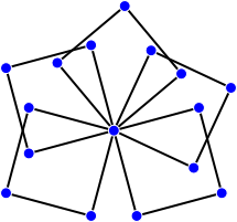
Suppose we have n possibly overlapping squares that share exactly one vertex (corner); in other words, there is one point that is a vertex of each of the squares, but no other point is a vertex of more than one square. The figure below shows one way to draw five such squares (i.e., this is the case n = 5). How many vertices do the squares have in all?
We begin by drawing some examples, counting the number of vertices, and constructing the following table. We are using the notation f(n) for the total number of vertices of n squares to emphasize that the number of vertices is a function of n, though we don’t know a formula for the function yet.
| n: | 1 | 2 | 3 | 4 | 5 | 6 |
|---|---|---|---|---|---|---|
| f(n): | 4 | 7 | 10 | 13 | 16 | 19 |
We would like to find a formula for f(n) in terms of n. In this case the pattern is fairly easy to see: each value of f(n) is 3 more than the previous value. We can see this if we look at the differences between successive numbers in the sequence, writing these differences in a row beneath the f(n) row.
| n: | 1 | 2 | 3 | 4 | 5 | 6 | ||||||
|---|---|---|---|---|---|---|---|---|---|---|---|---|
| f(n): | 4 | 7 | 10 | 13 | 16 | 19 | ||||||
| 3 | 3 | 3 | 3 | 3 | ||||||||
If we plot the points in our table, with n on the horizontal axis and f(n) on the vertical axis, we see that the points lie on a straight line. This leads us to guess that the function f(n) can be described by a linear polynomial, that is, a polynomial of degree 1.
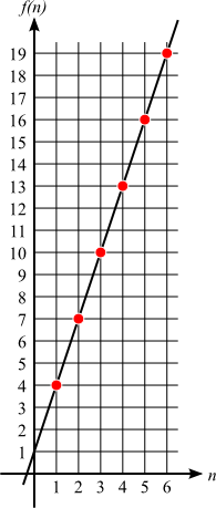
This line has a slope of 3 (the same 3 that is the common difference we saw above), so the equation of the line is f(n) = 3n + b for some value of b. One way to find the value of b is to know that it represents the y-intercept of the line; from our plot above, we see that b = 1.
Alternatively, we can choose a value of n that we know and the corresponding value of f(n), plug them into the incomplete formula f(n) = 3n + b, and solve for the value of b. Let’s use n = 1 and f(n) = 4. We get the equation
4 = 3⋅1 + b,
from which it is clear that b must be 1.
So our guess for the formula of f(n) is
f(n) = 3n + 1.
Let’s check this formula with the data we know. When n = 5, for example, we know that f(n) = 16 (from our experimentation). And our formula says
f(5) = 3⋅5 + 1 = 16,
so it seems to check out. You can check the other points from our table; they should agree with the values given by our formula.
Let’s try another problem. How many diagonals does a regular n-gon have? (Recall that a regular n-gon is a shape with n equal sides and n equal angles. A diagonal is a line from one vertex of the n-gon to another, except that edges of the n-gon don’t count.)
As before, we start by drawing some examples. The smallest value of n that makes sense is n = 3 (a 3-gon is a triangle); we continue up to n = 8 (an 8-gon is an octagon).
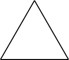

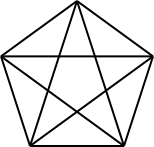
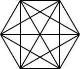
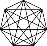
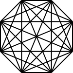
We see that a triangle has no diagonals, a square has two, a pentagon has five, a hexagon has nine, and so on. We record this information in a table, using n for the number of sides and d(n) for the number of diagonals. [We could have reused f(n), but since we already used the letter f with a different meaning earlier we chose a different letter this time. On the other hand, we are reusing the letter n with a different meaning here. It’s not terribly important what you name your variables; just be consistent within any one problem.]
| n: | 3 | 4 | 5 | 6 | 7 | 8 |
|---|---|---|---|---|---|---|
| d(n): | 0 | 2 | 5 | 9 | 14 | 20 |
As before, we’ll start by taking differences between successive terms of the sequence.
| n: | 3 | 4 | 5 | 6 | 7 | 8 | ||||||
|---|---|---|---|---|---|---|---|---|---|---|---|---|
| d(n): | 0 | 2 | 5 | 9 | 14 | 20 | ||||||
| 2 | 3 | 4 | 5 | 6 | ||||||||
This time we don’t have constant differences. But we notice that the differences themselves seem to have a pattern—each difference is 1 more than the previous difference. So, if we take the differences of the differences, we will get a constant row:
| n: | 3 | 4 | 5 | 6 | 7 | 8 | ||||||
|---|---|---|---|---|---|---|---|---|---|---|---|---|
| d(n): | 0 | 2 | 5 | 9 | 14 | 20 | ||||||
| 2 | 3 | 4 | 5 | 6 | ||||||||
| 1 | 1 | 1 | 1 | |||||||||
Since we had to take differences twice before we found a constant row, we guess that the formula for the sequence is a polynomial of degree 2, i.e., a quadratic polynomial. (In general, if you have to take differences m times to get a constant row, the formula is probably a polynomial of degree m.) The general form of a function given by a quadratic polynomial is
d(n) = an2 + bn + c,
where the coefficients a, b, and c are real numbers. In our case these coefficients are unknown; we are trying to find them. Since we have three unknowns, we will need a system of three equations. To get these equations, we can use some of the values of n and d(n) that we know. For example, plugging in n = 3, d(n) = 0 into the general quadratic d(n) = an2 + bn + c gives the equation
0 = a⋅9 + b⋅3 + c.
Similarly, plugging in n = 4, d(n) = 2 gives
2 = a⋅16 + b⋅4 + c,
and n = 5, d(n) = 5 gives
5 = a⋅25 + b⋅5 + c.
This gives us the following simultaneous system of three linear equations in three unknowns. (The numbers in parentheses to the left of the equations are simply labels so that we can refer to the equations; they are not part of the equations themselves.)
| (1) | 9a | + | 3b | + | c | = | 0 |
| (2) | 16a | + | 4b | + | c | = | 2 |
| (3) | 25a | + | 5b | + | c | = | 5 |
We can solve this system algebraically to find the values of the coefficients a, b, and c. (For a review of some useful algebraic techniques, see Appendix A in Problem Solving Through Recreational Mathematics.)
One way to solve a system of linear equations is to systematically substitute or eliminate variables one at a time until only one variable remains. Solving for the single remaining variable is easy, and then you can back-substitute the values of the variables you know to find the values of the variables that were eliminated.
Let’s start by solving equation (1) for c.
| (4) | c = −9a − 3b |
This gives us an expression to substitute for the variable c. If we plug this expression into the other two equations, (2) and (3), we get a simultaneous system of two linear equations in two unknowns.
| 16a | + | 4b | + | (−9a − 3b) | = | 2 |
| 25a | + | 5b | + | (−9a − 3b) | = | 5 |
After we combine like terms, we get the following system.
| (5) | 7a | + | b | = | 2 |
| (6) | 16a | + | 2b | = | 5 |
Now b looks like a good candidate to eliminate. If we multiply equation (5) by −2 and add it to equation (6), the b’s will cancel:
| −14a | − | 2b | = | −4 | |
| 16a | + | 2b | = | 5 | |
| (7) | 2a | = | 1 | ||
We have substituted or eliminated all but one variable, whose value we can now find. From equation (7) we see that a = 0.5. Now we begin the process of back-substituting the values of variables we know into previous equations in order to find the values of the other variables. We can plug the value a = 0.5 into equation (6), say, to get the equation
8 + 2b = 5,
so 2b = 5 − 8 = −3, which means b = −1.5. Now we know the values of both a and b, so we can plug them into equation (4) to get
c = −9(0.5) − 3(−1.5) = 0.
So we have found the coefficients of the quadratic polynomial: a = 0.5, b = −1.5, and c = 0. So we guess that the formula for d(n) is
d(n) = 0.5n2 − 1.5n.
Let’s check this formula with some data from our table, to make sure we didn’t make an algebraic error somewhere. We’ll try n = 8, for which we should get d(n) = 20:
d(8) = 0.5(82) − 1.5(8) = 20.
It checks out. Try a few more values of n and make sure this formula works for the data we have.
In the examples above, we looked at one sequence that was described by a linear (degree-1) polynomial, and another that was described by a quadratic (degree-2) polynomial. Some sequences might be described by polynomials of higher degree. A polynomial of degree 3 is called a cubic polynomial, one of degree 4 is called quartic, and one of degree 5 is called quintic; polynomials of degree higher than 5 aren’t usually given special names. Formulas for sequences described by such polynomials can be found using the technique described above; there will just be more algebra to do (but not harder algebra).
For example, if you are investigating a sequence described by a quartic (degree-4) polynomial, you will find that you need to take successive differences four times before you reach a constant row (this tells you the degree of the polynomial), and you will need to solve for five unknown coefficients, because the general form of a quartic polynomial (in the variable n) is
an4 + bn3 + cn2 + dn + e.
So you will need a system of five equations, which you can obtain (as we did above) by plugging in five sets of known values. Solving a system of five equations can be done just like solving a system of three equations; it just requires a bit more patience.
On the other hand, some sequences cannot be described by polynomials. For example, consider the sequence of powers of 2, given by the formula 2n:
| n: | 0 | 1 | 2 | 3 | 4 | 5 | 6 | 7 | 8 | 9 | 10 | … |
|---|---|---|---|---|---|---|---|---|---|---|---|---|
| 2n: | 1 | 2 | 4 | 8 | 16 | 32 | 64 | 128 | 256 | 512 | 1024 | … |
You can start taking successive differences of these numbers, but no matter how long you go, you will never reach a constant row. (Try it and see.) This sequence grows too quickly to be a polynomial sequence. It is an exponential sequence instead, meaning that the variable n is in the exponent in the formula 2n. The method described here will not work for sequences (like this one) that are not polynomial sequences. There are other methods that can be used to find formulas for certain types of nonpolynomial sequences, such as exponential sequences, but the details of such methods are probably beyond the scope of this course.
It is important to note that this method produces only a guess for a formula—it doesn’t actually prove that the formula is correct in general. For example, in the squares problem it is conceivable that the formula works only for values of n up to 6, and then fails after that; or maybe it works for all values of n up to a million, but doesn’t work for n = 1,000,001. We can test more values of n, drawing more and more squares, counting the number of vertices, and comparing this with the value predicted by the formula, but we won’t ever be able to test every possible value of n. So how can we be positive that the formula will always work?
This is the fundamental question that provides the inspiration for all of mathematics: How do we know that a guess is correct; how do we know it is always true? The answer lies in the concept of mathematical proof. When we guess a formula for f(n), we have made a conjecture, an educated guess based on a body of evidence. But it is not a theorem, an established mathematical fact, until we can provide a proof, a logical justification that explains why it must be always true. Proof is important; it is what separates statements that are known to be true from statements that merely seem to be true. Many conjectures that seem true at first turn out to be false when they are studied more extensively. It is not uncommon for a mathematician to make a conjecture and even announce it publicly (as a conjecture, of course), only to be proved wrong later by someone who finds a counterexample, an exception to the conjecture. This is part of the process by which mathematical knowledge grows and evolves.
Finding a proof for a conjecture can be difficult and may require a very creative way of looking at the problem. There are some conjectures in math that have eluded all attempts at proof for hundreds of years. On the other hand, many conjectures can be proved with just a bit of thought. A mathematical proof does not have to follow a strict format or be encrusted with strange-looking symbols; all that is required is an explanation following a careful, logical train of thought that shows why the conjecture must be true.
Let’s try to prove our conjecture that the total number of vertices in the squares problem is given by the formula f(n) = 3n + 1. We might first ask ourselves, “Why does the formula end with ‘+1’? What significance does that have? What does it correspond to?”
Let’s see if there is any single object that might give us the “+1” in the formula. Since the formula is counting vertices, the “+1” seems to point to one special “extra” vertex that has to be added in at the end. Looking at a picture, we might guess that the “+1” corresponds to the single vertex that is shared by all of the squares. If so, then the remaining vertices should be accounted for by the “3n.” Aha! The variable n represents the number of squares, and each square has 3 unshared vertices that are its own and do not belong to any other square. So the total number of these unshared vertices is given by 3n. To this we must add 1 for the shared vertex, giving us a total of 3n + 1 vertices in all, which is the formula we guessed.
Once a mathematician has figured out the idea for a proof, he or she usually rewrites the proof in a more succinct and polished form. (It is worth remembering this when reading a proof in a book—what you are reading is a final draft, with all of the messy trial-and-error thought processes that were required to produce the proof hidden. Nobody, not even an experienced mathematician, writes a complete, well-written proof from start to finish the first time they try.) A polished presentation of the conjecture we just proved (now a theorem!) might look like the following.
Theorem. The total number of vertices for n squares that share exactly one common vertex is given by the formula f(n) = 3n + 1.
Proof. Each of the n squares has 3 vertices that are not shared with any other square; this gives 3n unshared vertices in all. In addition there is a single vertex that is shared among all the squares. So the total number of vertices is 3n + 1.
Now that we have a proof for this theorem, we know that the formula f(n) = 3n + 1 always works. This is an amazing and beautiful thing. We have proved a statement that is true for infinitely many values of n—the formula for f(n) works for any positive integer n—even though we can never check every case one by one! So, for example, we now know with complete certainty that if a million squares share exactly one vertex, the total number of vertices is
f(1,000,000) = 3⋅1,000,000 + 1 = 3,000,001.
Of course we could never accurately draw this many squares and count their vertices by hand, but that’s not necessary to know that our answer is right.
Can you prove the formula we guessed for d(n), the number of diagonals of a regular n-gon? It is not easy to see what is going on when the formula is written as d(n) = 0.5n2 − 1.5n. But we can factor this expression and write it in a more suggestive form:
| d(n) = | n(n − 3) | . |
| 2 |
Why is this formula correct?